The incredible inner world of LLMs (II)

June 11, 2025

X-ray of a model

Let’s take a look at a model from the inside, physically. For that, we’ll use this one:

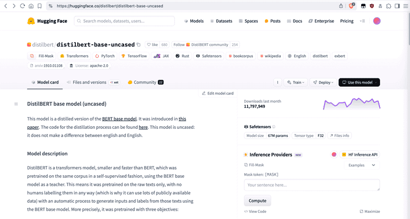https://huggingface.co/distilbert/distilbert-base-uncased

It’s a model (a distilled version of BERT) with a modest 67 million parameters. A bit old (in internet terms), but perfect for illustration purposes.

With a short script using the 'transformers' library (also from HuggingFace), we can download the model into the local directory:

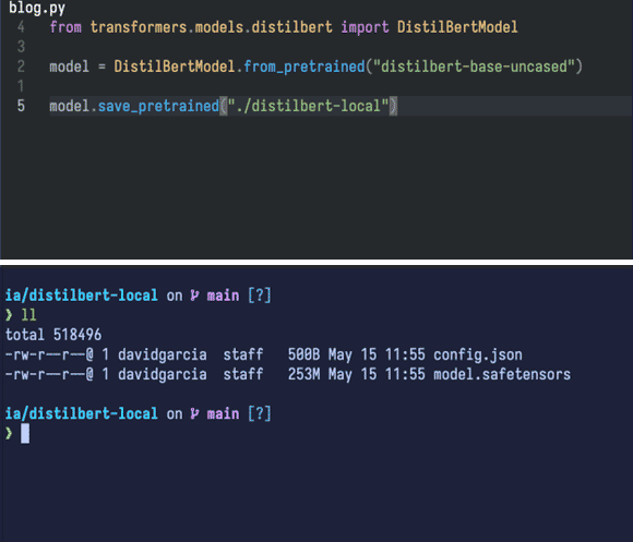
It downloads two files:

One is the model itself, model.safetensors (253 megabytes).
The other is config.json, which contains the model’s architecture—required for loading the model correctly with the library we’ll use (PyTorch).

This config.json file also provides us with a lot of valuable information.

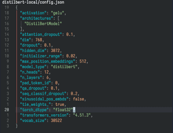
Let’s focus on some of the key data in that file.

Disk space required by the model’s vector space

The vocabulary size (vocab_size) the model 'understands' is 30,522 tokens:

Each of those tokens is associated with a vector (dim) of 768 'slots' or values. This vector is the same one we introduced at the beginning of the article, as a reminder:

TEF model: [1,1,1,1,1]
The piano: [0, 0.2, 0.8, 0, 1]

In other words, a position within a 768-dimensional vector space (keeping in mind that a Cartesian plane only has two).

Now, there’s another important point: each of those 768 data points in the vector space has float32 precision (torch_dtype), defining a unique token among the 30,522.

That float32 format means 4 bytes (or 32 bits). So, on disk, just the tokens require:

30,522 * 768 * 4 bytes = approximately 90 megabytes.

By the way, if you're curious to see the vocabulary of this model (the tokens), it’s available here.

Layers and parameters

Let’s not forget a key characteristic of neural networks: layers.

From the input layer, through the hidden layers, and out to the output layer, data flows and bounces across all the layers to produce the final result.

Our model under analysis has roughly 67 million parameters.

Just the embeddings layer (which holds the tokens and their associated vectors) contains:

30,522 * 768 = 23,440,896, around 23 million parameters.

We also need to add the parameters for each of the model’s layers. According to the "config.json" file, this model has six internal layers (the transformer model), indicated by the "n_layers" field.

In addition to those layer parameters, the model has others used to model bias, normalize values, and apply various tricks that help generate the final result: the model’s answer.

When you sum it all up, you reach that 67 million parameter count.

What does a model look like on the inside?

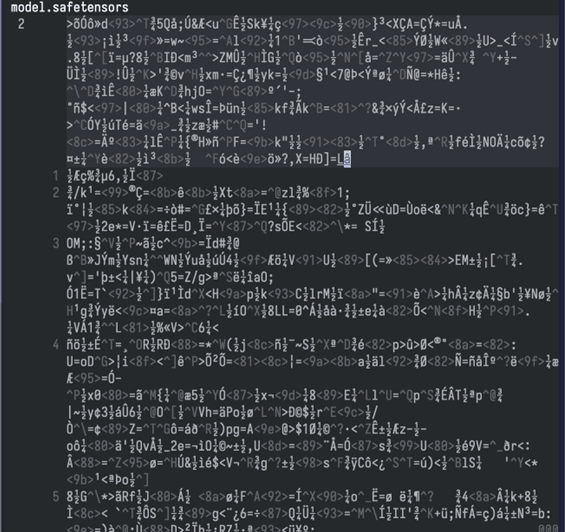
It’s a physical file (or sometimes a set of files). It includes a metadata field describing the internal structure, and the rest is binary data.

Let’s look at the metadata header:

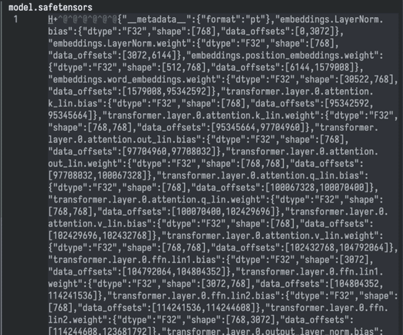
The rest of the file consists mainly of the weights of the different layers, in binary forma; naturally, unintelligible:

Using a small script with the safetensors library (also from HuggingFace), we can visualize what we discussed regarding the layers:

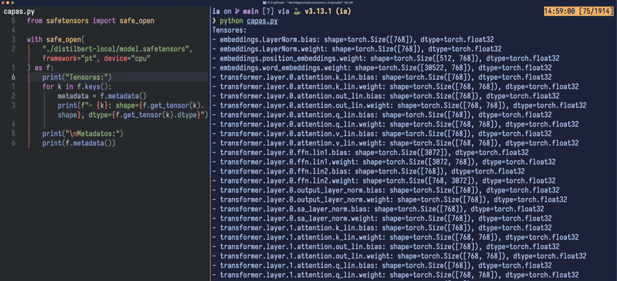
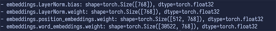
Take a look: we see the embeddings layer we examined earlier. With certain distributions (which may vary from one model to another), represented as tensors:

word_embeddings, easy to identify by its shape (30,522, 768), is a matrix (or 2D tensor) of 30,522 rows corresponding to the tokens, each with a 768-float32 vector; as indicated by the 'dtype'.
position_embeddings is another matrix, sized (512, 768). Note how important this is. When a phrase or paragraph is passed to the model as tokens, the model has no 'awareness' of their order. That’s why this space is used to organize the input.

That 512 value isn’t arbitrary: it’s the model’s maximum context length. Any input beyond 512 tokens will be truncated and not processed. It’s like the model stops listening after 512 tokens. Of course, it can process inputs in chunks (chunking), but… well, it’s not the same.

■ To give you an idea of modern context sizes: a model like Llama 3.2 1B or 3B has a context window of 128,000 tokens. Even Llama 4 Scout (though with more demanding requirements) can handle a context of 10 million tokens.

Context is critical for a model to understand what we’re asking it. The larger the context window, the higher the fidelity and quality of the response.

The elements shown as LayerNorm bias and weight are two vectors (1D tensors) with values learned during training. These are used to fine-tune (scale and shift) the output from the combination of word_embeddings and position_embeddings, just before the information enters the network layers.

Next, we see the actual layers—six in total, indexed from zero to five, all with the same types of tensors:

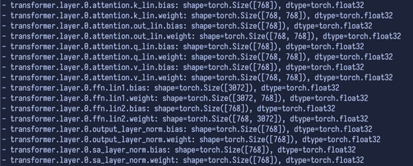
The first thing to understand is that all the tensors in the model are, essentially, either weights (weight) or biases (bias).

Weights are the major parameters the network learns during training. They act as the 'wiring' that transforms data from one layer to the next.
Bias is a type of 'fine-tuning' that adjusts each layer’s output ensuring, for instance, that even if the input is all zeros, the output can still be meaningful. It’s a subtle yet essential component.

So, each layer usually comes in pairs: a weight matrix and a bias vector to ensure proper performance in all situations.

We won’t go into every distinction, but one thing stands out: the label 'attention'. You’ve probably come across the phrase Attention is all you need. These are the parts of each layer that belong to the attention sub-layer or module.

Instead of processing text linearly (or sequentially), the attention mechanism—the core of the Transformer model—lets the model analyze the input (what we say) by interrelating all words simultaneously. It assigns each word a “score” based on the context, determining which to focus on more than others. A true revolution.

■ FFN is a familiar type of neural network: "Feed-Forward Network", which complements the attention mechanism. Thanks to the FFN, the model can focus (this time on a single token) and further refine the result coming from attention.

In fact, if we look at the iconic diagram from the famous paper, we’ll see FFNs play a key role as a model component:

Illustration 1 Transformer Model

Without this network, the model wouldn’t be able to detect complex relationships or nuances.

The rest consists of normalization layers that shape each layer’s output.

Bonus track: what happens if we progressively remove layers from a model?

Alright, let’s try it out. This is a model that replaces [MASK] with a word that fits the context.

We ask it:

> Madrid is located in:

First, let’s see it in action with all six of its layers:

It works correctly, guessing the word 'spain'.

Now we create a function that calls the model the same way, but progressively removes its layers...

■ As we can see, the output starts to go off track, since removing layers also reduces the model’s response accuracy. In upcoming articles, we’ll dive deeper into technical and practical aspects of large language models.

■ PARTE I