Neural networks: a historical and practical perspective (II)

April 14, 2026

In the previous article we introduced neural networks from a historical perspective. In this one, we will approach them from a practical perspective, with code we can actually 'touch'.

We will start with the simple Perceptron, introduced by Frank Rosenblatt, and use it to learn how to solve simple logical functions such as AND or OR.

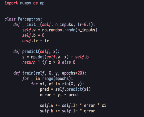
As we can see, we have a class Perceptron that includes a constructor and two methods, one for training (train) and another for making predictions (predict).

The logical functions AND and OR have two inputs (there can be more) and one output. These are the truth tables that map two values (the inputs) to a result:

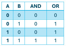
Therefore, the goal of our perceptron is to learn how they work and be able to solve the same problem on its own.

The goal: learn and generalise independently.

The value of the weights is generated randomly, as shown in the constructor (__init__) when using numpy.random.randn. If you look closely, the parameter n_inputs is defined by us when instantiating the class.

The main idea here is: if we have two inputs, then we will have two weights initialised randomly.

If the weights did not have random values, the neurons in a network would all learn exactly the same thing, adding no diversity to the learning process.

Bias and learning rate

The other two variables are the bias (self.b) and the learning rate (self.lr). The bias adds several positive features to the perceptron, including: better adaptation to input data, avoiding non activation when inputs cancel each other out (zeros) and, importantly, helping to prevent or mitigate overfitting and underfitting.

The bias improves model adaptation and stability

As we can see, it is also updated during training. The bias can be zero, an arbitrary value or even, like the weights, random. What matters is that it is adjusted during training like any other weight.

On the other hand, 'lr' (learning rate) measures how much the weights will be adjusted during training. In other words, the amount that will be added or subtracted (depending on the sign of the error) from the weight.

It is best understood as the temperature dial on an oven. If the learning rate were 0.1, each step of the dial would increase the temperature by 0.1 degrees, whereas if it were 0.001, each step would increase it by just one thousandth of a degree.

This greatly affects the outcome of training, since a small learning rate requires many iterations to reach a fine adjustment, while a large one may never reach an optimal adjustment due to being too coarse.

The artificial neuron and its activation

If you have never seen this before and imagined billions of interconnected points with lights flashing inside a hypercube in virtual reality... sorry to disappoint.

This is an artificial neuron:

It is the result of a weighted sum plus the bias. This value, stored in z, is the output of the neuron.

The line below is its activation function, which in this case is not even a function, just a simple if-else statement.

Disappointing, right? Well, if you strip away the complexity, you will find remarkable mathematical depth. Let us break it down.

A neuron is simple… its combination changes everything.

What we do is multiply the weight vector by the inputs and add the bias. This strongly resembles a very familiar mathematical object: the linear function. In fact, a neuron is exactly that. The real power lies in how they are combined into layers and how those layers interact.

Equally important is the activation function. This mechanism determines whether the neuron activates or not. It takes the final value computed by the neuron and checks whether it falls within the activation threshold.

There are several activation functions. The simplest one we are using here is the step function:

It is simple: we set a value and if 'z' is greater than it (exceeds the threshold), it activates; otherwise, it remains inactive.

The problem with this function is that it is so simple that its derivative is not useful for training a network with backpropagation.

For multilayer networks, we use functions that do allow this, such as ReLU, ELU or Softmax, among others.

Training

As shown in the code, there is a number of iterations defined by the parameter epochs.

This parameter indicates the number of training cycles or adjustments of the perceptron. In other words, how many times it will perform 'trial and error' and update its parameters.

Training means iterating: trial, error and adjustment

If the number is too low, there will be no convergence, the model will not fully train and inference results will be poor. In short, it has not had enough time to understand the problem.

If the number is too high, it becomes unnecessary because once the error rate reaches zero, the weights will no longer be updated.

This is easy to see in the code:

If the error is zero (note the multiplication), the adjustment is null.

At this point, we should pause: if the data is linearly separable (such as OR or AND), we will reach a state where the error rate is zero.

If, on the other hand, the data is not linearly separable (such as XOR), a single layer perceptron will never converge.

Not every problem can be solved with a simple perceptron.

No matter how much we increase the number of epochs or iterations, a single layer perceptron will not solve the problem because mathematically it cannot converge.

Demonstration

Let us train our perceptron to solve the AND function:

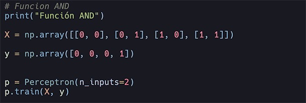
We set two parameters n_inputs and feed it all possible outputs for all possible inputs where n=2.

With our trained perceptron, we make predictions on possible inputs:

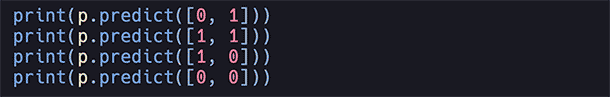
We execute it:

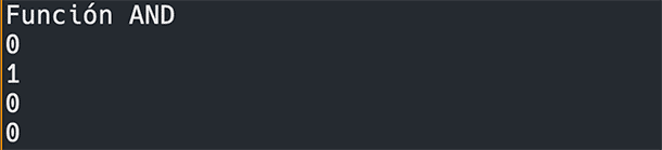
100% accuracy.

With linearly separable data, the model performs perfectly.

Now let us try to train the network to solve the XOR function, which, as mentioned, is not linear and therefore cannot converge during training:

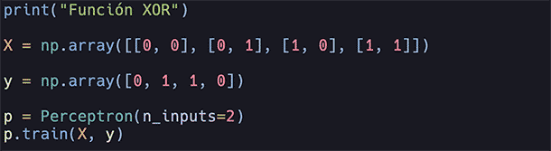
Model trained, let us execute it with:

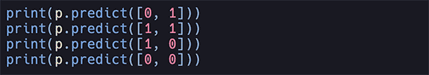
Result:

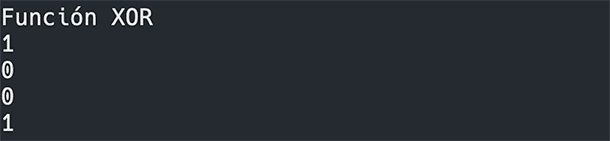
As we can see, it performs worse than random guessing.

Conclusion

The rise of neural networks may seem straightforward in hindsight, but it was not.

What we achieve today with just a few lines in one of the best programming languages was, in the 1960s, a demanding and complex task.

We have seen the basic functioning through the simplest neural network model: the perceptron, the pioneer that paved the way.

The next step is the era of the multilayer perceptron, which broke the barrier of non-linearity and led to the resurgence of neural networks thanks to backpropagation.

■ In upcoming articles, we will explore in practice how it emerged, how it works and how we can implement it.